Calibration as a Chain of Separate Checks

Why this matters

A PAUT setup can place one reference echo correctly while other laws remain shifted, weak or incorrectly positioned. That happens because “calibration” is not one property. Material velocity, wedge delay, law sensitivity, distance compensation and encoder scale answer different questions. This chapter follows a guided setup story from an uncorrected screen to an identified, checked configuration. Each stage states what changed, what the examiner should expect to see and what the change cannot prove. The result is a practical dependency chain rather than a menu recipe.

What you already need

• Echo time can be converted to distance only with the right path model and velocity.
• Wedge and material data influence focal-law timing and displayed position.
• A law group contains several beam conditions that may respond differently.
• An encoder has its own scale, direction, zero and offset.
• Response amplitude is not a direct measurement of flaw size.

What you will learn

• Separate service calibration, user setup calibration, reference sensitivity and performance checks.
• Match a reference target to the relationship being established.
• Put velocity, wedge delay, sensitivity and distance compensation in a sensible order.
• Explain the before-and-after screen effect of each calibration stage.
• State what each stage proves and what it cannot prove.
• Identify the equipment and setup details that belong to one calibration state.

Words you will meet

• Reference standard: a controlled block or feature used to establish a known relationship.
• Wedge delay: timing contribution between the array event and the selected component-surface reference.
• Sensitivity equalisation: law-by-law gain correction for a chosen reference response.
• DAC: a displayed distance-amplitude reference curve.
• TCG: gain applied with time or path to equalise selected reference responses.
• DGS: a method comparing response with modelled ideal-reflector behaviour.
• Residual error: the difference remaining after a correction is applied.

33.1 Calibration answers several different questions

The word calibration is often used for four related activities. They should not be treated as interchangeable.

Laboratory or service calibration checks instrument functions against traceable references at controlled intervals or after repair. It may address time base, gain or electronics. A certificate supports the instrument, but it does not validate one probe, wedge and focal-law setup.

User setup calibration or standardisation relates the assembled field system to known paths, positions and responses. It can include velocity, wedge delay, law sensitivity, DAC or TCG and encoder checks.

Reference sensitivity sets a repeatable artificial-reflector response for comparison. It does not establish the smallest natural flaw that will always be detected. Orientation, material, coupling, coverage and analysis still matter.

Performance or stability checks compare current behaviour with an accepted baseline to reveal change. They are examined in Chapter 34.

These activities can all pass while an inspection remains unsuitable for its component. Complete-system verification is one control layer, and application calibration is another. Standards scopes distinguish instrument, array-probe and complete-system characterisation, but their existence does not supply hidden universal tolerances or application proof. [R043] [R044] [R045]

33.2 Use a reference target for one declared purpose

No single block proves every PAUT property. A known radius or back wall can supply a known sound path. A side-drilled hole can provide a repeatable cylindrical response for comparison across laws or distances. A flat-bottom hole provides a flat circular face with strong orientation dependence. A notch can represent a controlled surface-connected reflector over the directions for which it is suitable.

Before interpreting a result, state the relationship the target is meant to establish. Examples include time zero, material velocity, a known path, law-to-law response, distance-amplitude behaviour, beam location or encoder travel. Then make sure the target position and orientation suit the laws and range being checked.

A side-drilled hole is not a crack of the same diameter. A smooth radius is not a flaw simulator. A notch that responds well at one angle is not automatically uniform across a wide sector. Reference targets are valuable because their geometry and position are controlled, not because they duplicate every service discontinuity.

The reference standard also needs identity. Material, dimensions, drawing revision, surface condition, temperature relevance and target orientation can affect the relationship. A textbook sketch helps the learner understand the feature but does not become a manufacturing drawing.

33.3 Follow the dependency chain

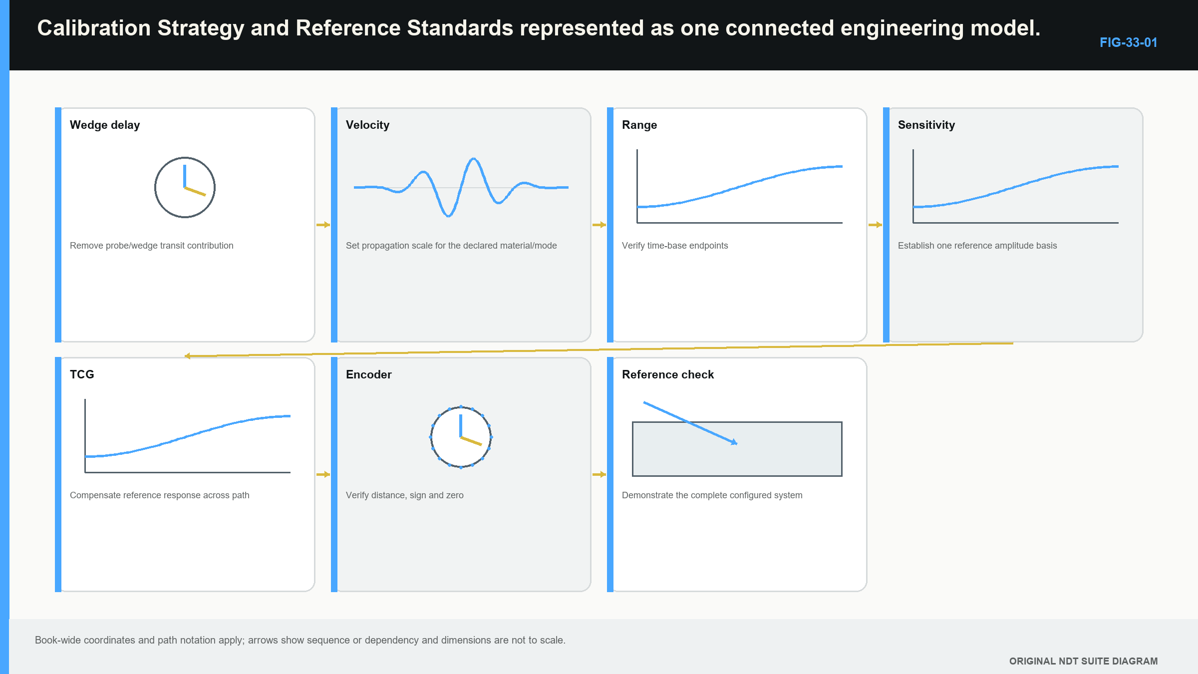
Calibration order matters because later corrections use earlier assumptions. A practical study chain is:

1. identify the component, examination volume, setup and reference targets;
2. confirm probe, wedge, element orientation and material inputs;
3. generate and review the required law groups;
4. establish material time-distance behaviour;
5. establish wedge and system timing for the included laws;
6. establish a chosen reference response across those laws;
7. establish response versus distance where required;
8. establish encoder scale, direction and offsets;
9. check the complete configuration on known independent features;
10. save and identify the accepted setup state.

This order is not a universal button sequence. Instrument interfaces vary. The dependency is the lesson. An amplitude correction built on the wrong velocity equalises the wrong beam geometry. Wedge-delay correction cannot repair a backwards probe. Encoder calibration cannot repair an incorrect acoustic offset.

The following figure shows the checks as a ladder. Each step supports particular later measurements, and the side labels state what remains outside its proof. [R042]

33.4 Guided setup story: begin before correction

Consider a shear-wave sector aimed at known reflectors in a reference block. Before applying corrections, inspect the screen. The expected reflector should appear on the relevant laws, but its indicated path may form a curved or sloping band. Amplitudes may vary across angle. These observations are useful because they reveal whether the basic law geometry and target interaction are plausible.

If some laws cannot see the target, do not immediately force them to the same level. The cause may be poor coupling, wrong probe orientation, an unsuitable target, weak steering, a damaged element or an incorrect wedge model. A calibration routine can only correct a valid observed relationship.

Confirm that the selected gate contains the intended echo and excludes competing responses. Confirm that signals are not clipped. Record which laws and path range the target actually supports. The “before” display becomes evidence of the corrections being asked to act.

The same principle applies after every stage. Look for the expected change, measure the residual difference and check an independent feature where practical. A wizard completion message is not a physical observation.

33.5 Material velocity: set the time-to-distance scale

Material velocity tells the setup how ultrasonic time relates to travel in the selected wave mode. It affects displayed path and, when used in law calculation, refracted direction and focus. Velocity can vary with mode, composition, structure, temperature and propagation direction.

A robust comparison uses one or preferably two known paths in representative material. Two separated echoes help distinguish propagation time from a fixed system or wedge delay. The selected echoes must belong to the same represented mode.

Before adjustment: known reflectors can be increasingly displaced as path grows. The spacing between two known echoes does not match the physical spacing.

After adjustment: their relative spacing agrees more closely over the checked range.

What this establishes: a working time-distance relationship for the stated material, mode, direction and conditions.

What it does not establish: correct wedge geometry, correct element order, complete coverage, law sensitivity or detection capability.

If the velocity used to calculate focal laws changes materially, rebuild the affected laws before continuing. A later delay shift can move echoes along the time axis but cannot restore the refracted direction calculated from the wrong velocity.

33.6 Wedge delay: align a known path across laws

Each selected element has a path through the wedge before sound enters the component. Different apertures and angles can have different wedge travel contributions. Wedge-delay calibration applies timing corrections so a known reflector appears at its correct path or depth for the included laws.

Before correction: the same known target may appear as a curved band across the sector. Some laws report too long or too short a path even though their response is repeatable.

After correction: the target band aligns more closely with the declared known path, and the residual error lies inside the controlled limit for the included range.

What this establishes: the timing offset relationship between the assembled probe-wedge-system and a known target over the checked laws.

What it does not establish: correct material or wedge velocity, correct wedge angle, focus quality, beam coverage or equal sensitivity. It also cannot repair a worn wedge that rocks unpredictably.

When correction fails to make a stable target align, investigate the target identity, echo selection, element order, wedge data, coupling and law model. Repeating the same routine with more enthusiasm tends to calibrate the confusion rather than the system.

The basic pulse-echo relationship includes the fixed delay explicitly:

The subtraction comes before the division by two because fixed delay is not travel to and from the material reflector.

33.7 Law-to-law sensitivity: compare one chosen response

Even after timing is aligned, the same reference target can produce different amplitudes across laws. Element response, wedge path, angle, aperture and transmission all contribute. Law-to-law sensitivity correction applies gain offsets so the chosen target reaches a common reference band.

Before correction: a valid target envelope rises and falls across the included laws. Extreme or abnormal laws may stand apart.

After correction: the chosen target responses lie closer to the stated level, with recorded per-law offsets and remaining variation.

What this establishes: a common response from one selected reference target under the calibration conditions.

What it does not establish: equal response from every real discontinuity, missing-beam coverage, minimum detectable flaw size or correct distance compensation. A planar crack facing one beam differently from another will not obey the artificial-target equalisation.

Large or irregular offsets are diagnostic information. They may indicate weak steering, poor target interaction, damaged elements or a competing echo. Automatic normalisation should not be allowed to hide the original pattern.

33.8 DAC, TCG and DGS answer distance questions differently

Response from a comparable reflector often changes with path because the beam, attenuation and system transfer change. A DAC curve plots selected reference responses at several paths. The curve remains visible, and indication response is compared with it according to the approved method.

TCG applies gain with time or path so those selected reference responses approach a common screen level. TCG can make comparison through the range easier, but far-range gain can raise noise or cause clipping. Its reference points need to cover the valid range.

DGS compares a response with idealised reflector behaviour and may express an equivalent reflector size. That result is a model-based acoustic comparison. It is not a direct measurement of the physical discontinuity diameter.

Before distance compensation: equal reference targets at increasing paths commonly show different amplitudes.

After DAC or TCG work: the reference relationship is represented by a curve or an applied gain profile over the stated range.

What this establishes: how the chosen reference responses are treated with distance under the selected method.

What it does not establish: real-flaw equivalence, correct coverage or reliable sizing outside the qualified method. The governing document decides which method and comparison rule applies.

33.9 Encoder and position checks remain separate

After acoustic timing and sensitivity are established, position recording still needs its own evidence. Move the scanner through a known representative distance, verify scale, confirm positive direction and test return or reverse behaviour as required.

Before correction: a known mark may appear stretched, shifted or mirrored in the encoded display.

After correction: the known travel and direction agree within the controlled limit, and the probe-to-datum offset places a known feature correctly.

What this establishes: scale and direction under the check conditions, plus the declared offset when that feature is tested.

What it does not establish: stable wheel traction over the whole component, correct beam geometry, full law-set storage or valid coupling. Those are checked through acquisition trials and performance monitoring.

33.10 Identify and preserve the accepted setup state

Calibration belongs to an identified system, not just a filename. The state includes instrument and software, probe, wedge, cable and adaptors; pulser, receiver, filter, rectification and averaging; material and wedge velocities; element orientation and geometry; group definitions and law ranges; reference targets; scanner and encoder; and environmental conditions when relevant.

Changes have different effects. Replacing a wedge can change delay, position, transmission and laws. Changing an amplitude filter can affect sensitivity and DAC or TCG while leaving encoder scale untouched. Reversing the probe changes element orientation and coordinates. The effect determines which relationships need to be re-established.

Final verification uses known features to challenge the complete setup without pretending to prove every application outcome. Save the configuration with a unique controlled identity and link it to the observations, targets, included laws, residual errors and valid ranges.

Formal release authority, acceptance tolerances and recheck intervals belong to the controlled quality system and later governance chapters. The Level 2 learning outcome is to state clearly what physical relationship each calibration established and what remains unproven.

Read the completed screen as a chain of evidence

Return to the sector used at the beginning of the chapter. The known reflector now lies at the expected path across the included laws. Its chosen reference response is inside the required band, and the distance-amplitude relationship covers the intended range. A known encoder mark also appears at the correct scan coordinate.

Those observations are stronger together than one completion message, but they still answer separate questions. Correct path supports timing. Similar selected-reference amplitude supports law equalisation. Correct distance behaviour supports the chosen DAC or TCG relationship. Correct scan coordinate supports encoder scale and offset.

Check a feature that was not used to create each correction. An independent path can reveal a velocity or delay combination that fitted one target but not the range. An intermediate amplitude target can reveal an implausible distance correction between entered points. A second physical position can reveal a coordinate offset hidden by the zero mark.

Then inspect the edges. Review the lowest and highest used angles, nearest and farthest paths, and first and last aperture positions. A calibration that is strong in the middle can still leave unsupported edge laws. Record exclusions rather than allowing the word “complete” to hide them.

Finally, save the identified state and reopen it. Confirm that probe orientation, group count, law ranges, gates and corrections survived the save. The exercise is not software administration; it checks that the evidence remains attached to the same configured measurement system.

If a later check shows a different result, return to this chain rather than recalibrating everything without diagnosis. Stable timing with changed amplitude points toward a different dependency from changed timing with stable amplitude. A position shift confined to encoded axes belongs to another branch again. The separated calibration story therefore becomes a troubleshooting map as well as a setup record.

Do not use the same word “offset” for every correction. Timing offset belongs to echo time, amplitude offset belongs to law sensitivity, and positional offset connects the probe or scanner to the datum. Naming the quantity prevents a correct number from being applied to the wrong part of the setup.

The same discipline applies to “range.” It can mean the displayed time span, valid calibrated sound-path interval, law angle range or component examination range. State which range was checked. A calibration may cover the screen while excluding some focal laws, or cover every law at one path while not covering the far evaluation distance.

In plain words

• Calibration is a chain of separate physical relationships, not one pass button.
• Reference targets are selected for a declared purpose and range.
• Velocity establishes material time-to-distance behaviour.
• Wedge delay aligns fixed timing contributions after geometry and velocities are credible.
• Law sensitivity equalises one chosen reference response across included laws.
• DAC and TCG represent response versus distance in different ways.
• Encoder scale and direction remain separate from acoustic calibration.
• Every accepted result belongs to an identified complete setup state.

Key terms

Reference standard; service calibration; setup calibration; reference sensitivity; velocity; wedge delay; residual error; sensitivity equalisation; DAC; TCG; DGS.

Key relationships

• known paths and echo spacing -> material velocity check;
• measured time - fixed delay -> material round-trip time;
• known target path across laws -> wedge-delay residuals;
• chosen target amplitude across laws -> sensitivity offsets;
• chosen target response across distance -> DAC or TCG relationship;
• known physical travel -> encoder scale and polarity evidence.

Common mix-ups

• Service calibration does not validate one inspection setup.
• Wedge delay cannot correct wrong velocity or geometry.
• Law equalisation does not prove equal response from real discontinuities.
• TCG does not convert echo amplitude into physical flaw size.
• A completed wizard is not the same as observed acceptance evidence.

Bridge to Chapter 34

Chapter 34 treats the accepted setup as a baseline and looks for change. It begins with visible symptoms—weak elements, shifted time base and stretched position—then links each symptom to a check and its possible consequence for data.

Sources and further study

• [R042]
• [R043]
• [R044]
• [R045]