Inside a PAUT System

Learning outcomes

After completing this chapter, the learner should be able to:

1. trace an ultrasonic signal through a generic phased array system;
2. explain the roles of the pulser, receiver, analogue front end, ADC, beamformer, gates, storage and display;
3. describe how transmit and receive delays form a focal law;
4. interpret common transmit:receive channel nomenclature without assuming that every manufacturer uses it identically;
5. distinguish pulse repetition frequency, complete-law-set acquisition rate and display refresh rate;
6. calculate a simple theoretical acquisition rate and relate it to scan increment and travel speed;
7. identify the assumptions and practical limits behind those calculations.

Key terms

Pulser: The circuit that supplies a controlled electrical excitation to selected probe elements.

Receiver: The signal path that accepts returning element signals and prepares them for beamforming and measurement.

Analogue front end: The amplification and filtering stage applied before analogue signals are digitised.

Analogue-to-digital converter (ADC): The circuit that samples an analogue voltage and represents each sample numerically.

Beamformer: The part of the system that applies channel delays and combines element signals to form the response for a focal law.

Focal law: The programmed transmit and receive timing used to create one beam condition.

Group: A set of laws and associated settings used for one inspection function within a setup.

Pulse repetition frequency (PRF): The number of pulse/receive cycles initiated per second under the stated convention.

Acquisition rate: The number of complete required law sequences acquired per second.

Display refresh rate: The number of times per second the visible screen is redrawn. It is a user-interface quantity, not proof of stored-data density.

Gate: A selected time or sound-path region in an A-scan used for detection, measurement, recording or triggering a derived value.

3.1 The system as a controlled signal path

A phased array instrument is easier to understand when it is treated as a chain of functions rather than a collection of menus. The chain begins with the inspection setup and ends with stored measurements and displayed information.

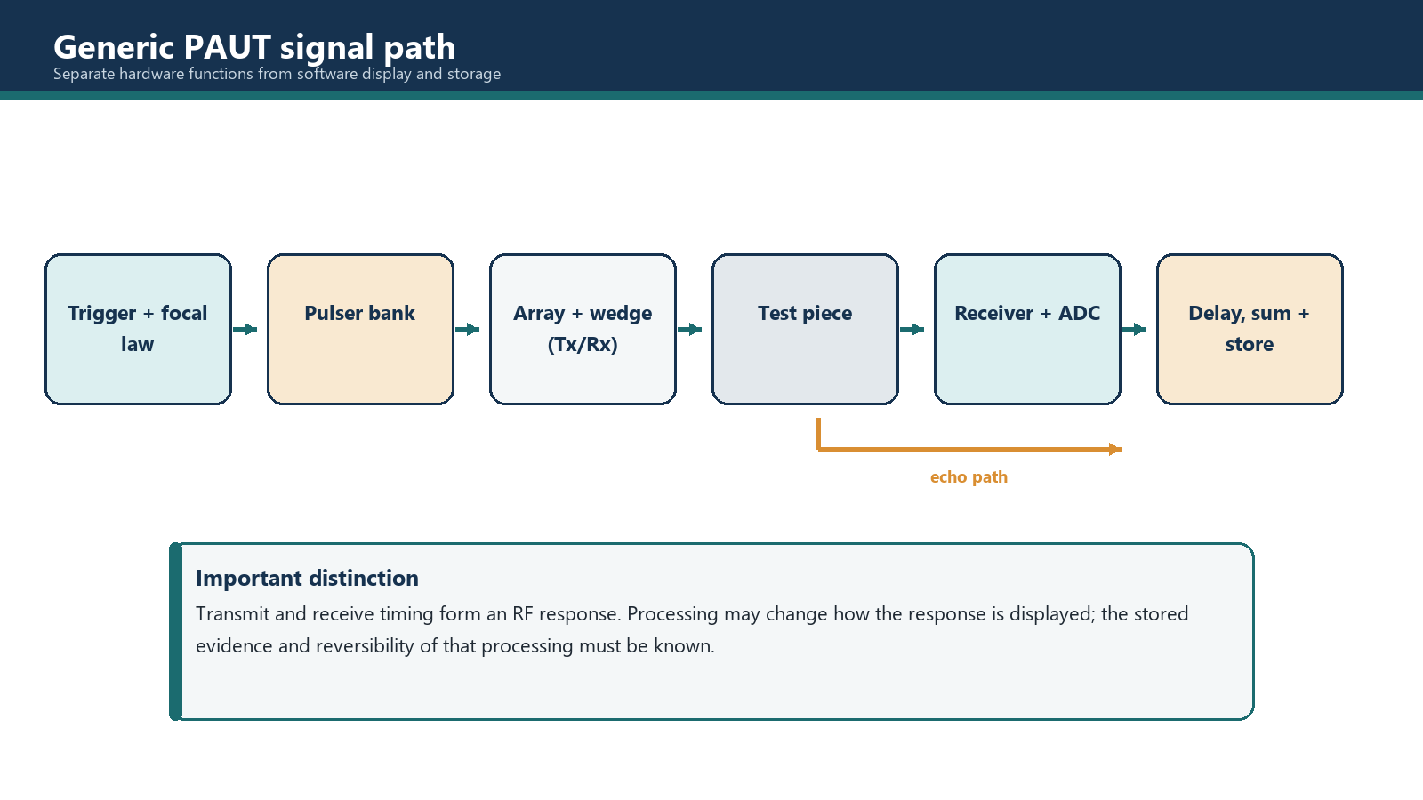
In a common digital beamforming architecture, the sequence is:

1. The setup defines the probe, wedge, material, aperture, angle or focus and the required law order.
2. The controller triggers the selected pulsers using the transmit delays for one focal law.
3. Excited elements convert the electrical pulses into mechanical vibration.
4. Wave components enter the wedge and component and combine into the intended beam.
5. Returning sound reaches the array elements at different times.
6. Each received channel is amplified and filtered in the analogue front end.
7. Each channel is sampled by an ADC.
8. Digital receive delays align the samples associated with the intended beam path.
9. The delayed channel signals are summed to create the A-scan response for that law.
10. The system applies the selected processing, gates and measurements, associates encoded position where applicable, and stores or displays the result.

Instrument designs vary. Some functions may be implemented in different hardware stages, and an operator should not infer the internal architecture from the screen alone. The important control principle is that the documented signal path must apply the required channel timing and produce a traceable response for every law used in the inspection.

Basic functions retained from conventional UT

PAUT still needs familiar ultrasonic functions:

• Gain controls amplification of received signals.
• Time base or range defines the part of the returning time history represented in the A-scan.
• Pulser settings control electrical excitation within the limits of the instrument and probe.
• Receiver settings may include analogue or digital filtering, rectification and other processing.
• Gates isolate selected response regions for measurement and recording.

The presence of many channels does not remove these controls. It repeats and coordinates them across a law sequence.

3.2 Acquisition unit, probe and movement system

The acquisition unit controls pulsing, reception, beamforming, digitisation, measurement, data handling and the user interface. It may be a portable instrument, a computer-controlled module or part of a larger automated system. This chapter remains vendor-neutral because the physical functions matter more than the colour and location of a particular button.

The probe contains the array elements. A wedge or delay arrangement couples the probe to the component and establishes the incident geometry. Probe and wedge parameters are used when calculating the delays and spatial corrections. Incorrect geometry or velocity data can therefore affect beam angle, focus, exit position and displayed location.

Movement can be manual, mechanically guided, semi-automated or automated. An encoder adds position information. It does not steer the ultrasonic beam and it does not verify coupling. Its job is to describe where the movement system was when the associated data was acquired.

The complete inspection system also includes the reference blocks, couplant delivery, scanner mechanics, cables, storage media and reporting path. A fault in any one of those can invalidate data produced by an otherwise healthy acquisition unit.

3.3 Forming a beam with delays

If all elements in a flat linear aperture are excited at the same time, their wave components tend to combine into a beam normal to the array face, subject to the probe and interface geometry. Applying progressively different delays changes where the components reinforce one another.

On transmission, the system delays the excitation of individual elements so that their wavelets arrive in phase along the intended wavefront. On reception, an echo from the intended direction or focal region reaches the elements at different times. The receiver applies corresponding delays before summation so that those contributions reinforce each other.

The combined response is an A-scan for one focal law. The system can then execute another law with a different angle, aperture position or focal setting. Repeating the sequence quickly creates the data used by phased array presentations.

A focal law is therefore more than an angle value. Its calculation depends on the declared probe element positions, wedge geometry and velocity, component velocity, wave mode, aperture and desired beam condition. A calibration can correct selected measurement offsets or sensitivity differences, but it cannot make fundamentally wrong probe, wedge or material inputs become correct.

3.4 Sequencing laws and groups

Two common uses of a law sequence are:

• Angle sequence: The same aperture is used with different delays to create a range of beam angles. This supports a sectorial or azimuthal presentation.
• Aperture sequence: A similar beam condition is moved along the array by changing which elements form the active aperture. This supports an electronic linear sequence.

A setup may contain more than one group. For example, one group may use a range of shear-wave angles while another uses a fixed-angle electronic sequence. Groups may share an array, use different apertures or be assigned to different probes. The instrument still has to execute every required pulse/receive cycle in the acquisition sequence.

Multigroup capability is useful, but it consumes timing and storage resources. When another group is added, the operator must consider the total number of laws, required PRF, available acquisition rate, file size and whether the instrument interleaves or otherwise schedules the groups. The simple equations in this chapter assume sequential laws with no extra overhead; actual performance must be confirmed on the equipment.

3.5 Understanding channel nomenclature

Phased array instruments are often described using a transmit:receive notation such as 16:64 or 32:128. In one commonly used convention:

• the first number indicates the maximum number of pulser channels available together for an active aperture;
• the second number indicates the larger set of element or receiver paths available for addressing and sequencing.

Under that convention, a 16:64 unit can form an aperture using up to 16 channels at one time and can sequence that aperture across as many as 64 addressable positions or elements, subject to the probe and instrument design.

This notation is useful, but it is not sufficient to define the instrument. The operator must also check:

• whether transmit and receive channel limits are identical;
• the maximum supported probe element count;
• whether channels are shared between groups or connectors;
• the permitted aperture size and law count;
• how total PRF is specified;
• whether full matrix, pitch-catch or other modes change the channel requirement.

Do not infer performance from a model label alone. Manufacturer documentation for the actual hardware and software configuration remains the authority.

3.6 PRF: the pulse/receive cycle rate

Each law needs enough time for its pulse to be emitted and for the required returning sound to be received before the next cycle creates interference. In its simplest form:

PRF = 1 / T_beam

where:

• PRF is in hertz (cycles per second);
• T_beam is the time allocated to one pulse/receive cycle in seconds.

This is a theoretical relationship. The usable setting may be lower because of range, slow sound velocity, multiple reflecting surfaces, wedge paths, instrument switching time, processing overhead, multigroup sequencing and the need to prevent echoes from an earlier pulse appearing in a later acquisition.

A high PRF is not automatically better. If sound from one pulse remains in the component or returns through a long path after the next pulse has begun, the later A-scan may contain a ghost response. The selected PRF must allow the relevant acoustic energy to clear under the inspection conditions.

Worked example 3.1 - pulse window and theoretical PRF

Assume a setup allocates 250 microseconds to one complete pulse/receive window.

1. Convert to seconds: 250 microseconds = 0.000250 s.
2. Apply PRF = 1 / T_beam.
3. PRF = 1 / 0.000250 = 4,000 Hz.

The result is a theoretical ceiling of 4,000 pulse/receive cycles per second before allowing for other timing constraints. It is not permission to set 4,000 Hz on every component with that displayed range.

3.7 Acquisition rate: complete law sequences per second

PRF counts individual pulse/receive cycles. An image or encoded position normally requires a complete set of the laws assigned to that acquisition. If N_laws are executed sequentially and every law uses an equal cycle time, then:

T_total = N_laws x T_beam

Acquisition rate = 1 / T_total

Combining those relationships gives the simple theoretical maximum:

Acquisition rate_max = PRF / N_laws

Assumptions:

• laws are fired sequentially;
• each law uses the same pulse/receive duration;
• no group-interleave, switching, processing or storage overhead is included;
• the stated PRF is the aggregate law-cycle PRF used in the calculation.

Actual instruments may report or limit these quantities differently. The operator must verify the displayed definition and the achieved acquisition status.

Worked example 3.2 - law count and acquisition rate

A group contains 48 laws. The aggregate PRF is 2,400 Hz.

Acquisition rate_max = 2,400 / 48 = 50 complete law sets per second.

The instrument can theoretically acquire the full 48-law group 50 times each second. It is not acquiring each law set 2,400 times per second.

3.8 Connecting acquisition rate to scan speed

For position-encoded acquisition, the required complete-law-set rate depends on travel speed and the distance between stored positions.

Required acquisition rate = scan speed / scan increment

with consistent units. If speed is in mm/s and increment is in mm, the result is acquisitions per second.

The corresponding simple speed limit is:

Theoretical maximum scan speed = available acquisition rate x scan increment

Worked example 3.3 - data spacing and travel speed

Continue Example 3.2, where the theoretical available acquisition rate is 50 sets/s. The planned scan increment is 0.8 mm.

Theoretical maximum speed = 50 x 0.8 = 40 mm/s.

If the operator plans to scan at 30 mm/s:

Required rate = 30 / 0.8 = 37.5 sets/s.

The theoretical 50 sets/s exceeds the 37.5 sets/s requirement. A real procedure should still apply an operating margin and verify that the instrument is not dropping data. Mechanical variation, processing overhead and brief overspeed can consume the apparent margin.

If the increment is reduced to 0.4 mm while speed remains 30 mm/s, the required rate doubles to 75 sets/s. If the instrument remains limited to 50 sets/s, the simple theoretical speed limit becomes 20 mm/s. Finer spatial sampling does not magically create more acquisition capacity; it demands more complete data sets per unit travel.

3.9 Display refresh rate is a separate quantity

The display refresh rate is how often the visible interface is redrawn. The instrument may acquire and store complete law sets faster than it can render them on screen. It may also average, skip or decimate visual updates while continuing to record according to the configured encoder increment.

For example, a system could store 50 complete law sets each second while refreshing the display 20 times per second. The visible motion may look less smooth than the stored position sequence, but the display rate alone does not prove that data is missing. Conversely, a smooth 60 Hz display does not prove that every required encoded position contains a complete law set.

Data integrity should be checked using the acquisition status, overspeed or dropped-data indication, encoded data pattern and the procedure's verification method. Judging completeness by how lively the screen looks is a surprisingly elegant way to inspect the user interface instead of the component.

3.10 Gates, measurements and stored results

A gate defines a region of the A-scan used for a purpose such as detecting a threshold crossing, finding a peak, measuring time or sound path, recording amplitude, or creating a derived B- or C-scan value. Gate start, width, threshold and measurement mode affect the reported result.

The operator should know whether a measurement uses the leading edge, peak, crossing point or another rule. Changing that rule after calibration can change the displayed location or amplitude basis. The same gate settings must be suitable for all laws and depths to which they are applied, or the setup must provide controlled alternatives.

Some systems store full waveform data; others store selected gated values, compressed representations or a combination. The distinction matters for later review. A colour pixel derived from a gate cannot always be expanded back into the original per-channel information.

Common traps

• Using PRF and acquisition rate as synonyms. PRF counts individual law cycles; acquisition rate counts complete required law sequences.
• Calling display refresh the data rate. A redrawn screen is not an encoded acquisition record.
• Calculating speed from increment without a complete-law-set rate. Both are required.
• Ignoring total laws across groups. Every required cycle consumes timing capacity.
• Treating the simple PRF/law formula as guaranteed instrument performance. It excludes switching, processing and storage overhead.
• Raising PRF to cure overspeed without checking acoustic clearance. This can introduce ghost echoes.
• Assuming channel notation is universal. Confirm the manufacturer's definition and actual connector/channel allocation.
• Changing gate measurement mode after calibration. The reference position used by the measurement may change.

Chapter summary

A generic PAUT system controls selected pulsers, receives element signals through an analogue front end, digitises each channel, applies receive delays and summation, and produces an A-scan for each focal law. Law sequences can change angle, aperture position or focus, and multiple groups can serve different inspection functions.

Transmit:receive notation describes channel capability under a declared manufacturer convention, but it does not fully define an instrument. PRF describes pulse/receive cycles per second. Acquisition rate describes complete required law sets per second. Display refresh rate describes screen redraws. These quantities may be related, but they are not interchangeable.

For a simple sequential sequence, maximum acquisition rate is PRF divided by total laws. Position-encoded acquisition then requires a rate equal to scan speed divided by scan increment. Real setups need operating margin and equipment verification because simple equations omit overhead and acoustic complications.