
CHAPTER 21 · Ultrasonics Level 3
Instrument Performance and Digital Signal Integrity
In this chapter · 20 sections
Why this matters
A Level 2 technician can recognise a flattened echo, an unstable time reading or a gap in encoded data; the Level 3 responsibility is to determine which instrument property caused the symptom and which results may have been affected. A self-test can pass while the receiver clips large signals, a time scale drifts with range, a filter moves a selected peak, or a buffer drops records during a fast scan. Digital storage preserves numbers exactly only after the system has captured the right signal, at the right time and position, with enough context to interpret it.
What you already need
- A-scan range, gain, gate, filter and pulse-repetition-frequency controls.
- Pulse-echo distance and simple time-to-distance conversion.
- The practical meanings of noise, saturation and reference response.
- Basic sample-rate and encoded-position concepts.
- The difference between electrical, acoustic and complete-system checks.
What you will learn
- Link visible instrument symptoms to timing, amplitude and digital mechanisms.
- Separate time offset, time-scale error, jitter and waveform-selection error.
- Explain linearity, clipping, noise and usable dynamic range.
- Assess filter, sampling and pulse-repetition effects on a measurement.
- Detect missing or transformed data that can weaken coverage evidence.
- Design an investigation using independent reference layers.
Words you will meet
- Horizontal linearity: consistent representation of time intervals across range.
- Vertical linearity: consistent representation of amplitude changes.
- Jitter: variation in timing relative to a stated reference.
- Dynamic range: span between usable lower and upper signal limits.
- Clipping: flattening caused when a signal exceeds a system limit.
- Group delay: frequency-dependent delay introduced by a wave or processing chain.
- Aliasing: false lower-frequency representation caused by inadequate sampling protection.
- Throughput: rate at which records can be acquired, moved and stored.
- Checksum: digital value used to detect a change in file content.
- Reversible: capable of restoring the prior data without information loss.
Depth guide for this chapter
- Understand here: visible error signatures, layered checks and decision consequences.
- Calculate here: timing sensitivity, linear time error, ideal pulse repetition frequency (PRF) range and spatial gaps.
- Derive later: filter theory, sampling proofs, effective-bit models and digital signal processing (DSP) estimators are developed in Chapters 64, 69 and 80.
21.1 Begin with visible symptoms
Instrument performance is multidimensional; a useful diagnosis starts with what changed on the screen or in the data, then selects a check that separates possible causes.
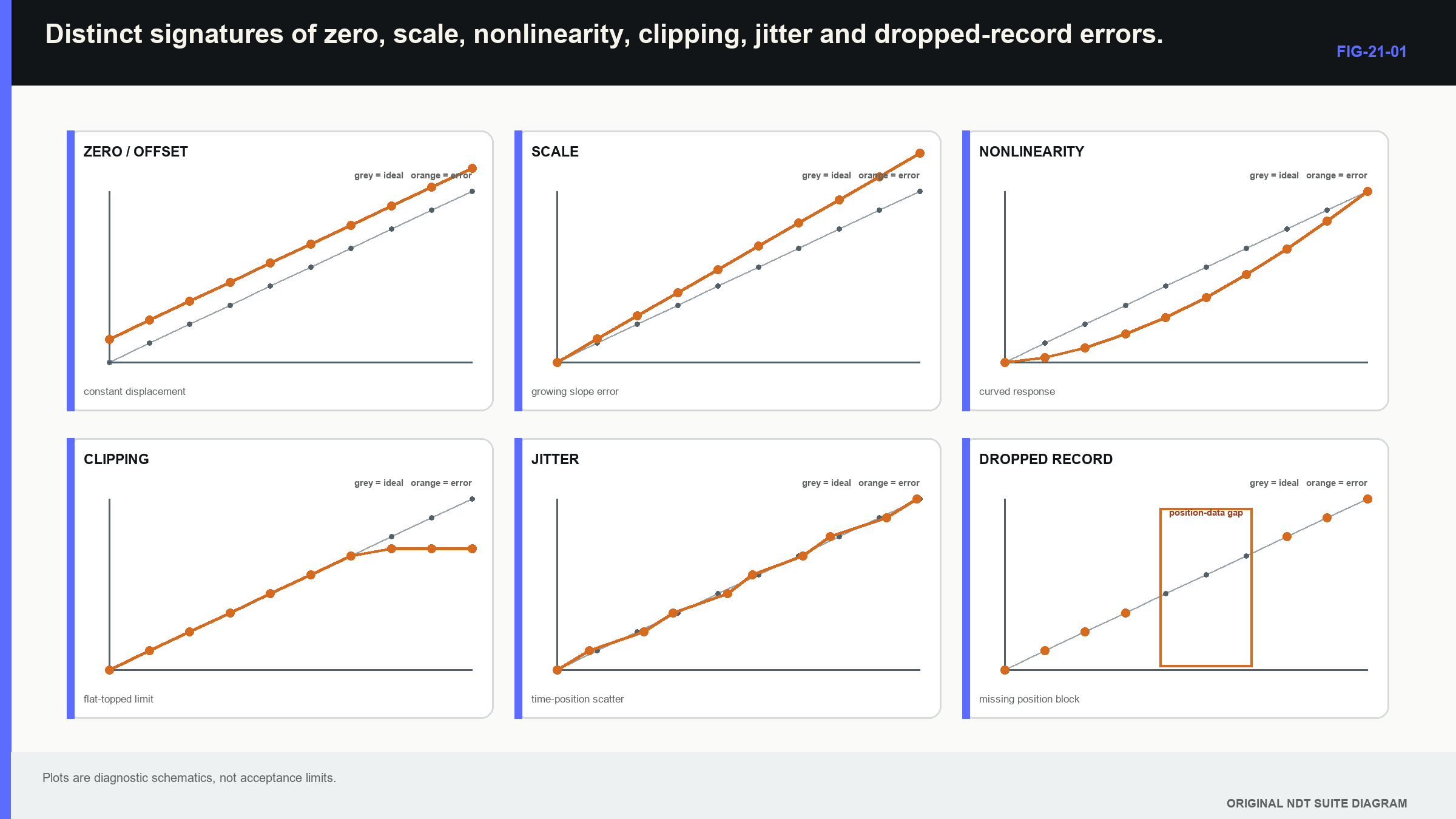
- A constant time shift across range suggests zero or trigger offset.
- A time error that grows with range suggests clock-scale error.
- Scattered time readings suggest jitter, unstable waveform or coupling.
- Flat-topped signals suggest receiver, converter or display clipping.
- Incorrect amplitude ratios suggest nonlinearity, compression or processing.
- A weak signal following a large echo suggests recovery or ring-down limits.
- Regular spatial gaps suggest trigger, buffer or throughput failure.
- A response changed only after reprocessing suggests software or filter identity.
These signatures are not final diagnoses; coupling can also move a waveform, and a selected peak can jump cycles. The purpose of the symptom list is to choose the next reference. Electrical injection tests much of the receiver and time base. An acoustic reference adds cable, pulser, probe and coupling. A coordinate reference adds scanner and encoder. The following figure places the main error signatures side by side; notice that offset, scale, nonlinearity and missing data produce different patterns even when each can be described loosely as an instrument error.
Instrument, probe and complete-system tests have different boundaries; current standards families distinguish those layers, reinforcing that a pass at one layer does not prove application capability at another. [R043] A boot-up self-test is evidence about whatever the manufacturer included in that test, not about the probe, component or target response.
21.2 Timing error in plain and formal terms
Horizontal accuracy describes how the instrument represents time; four effects should remain separate. A time offset adds nearly the same delay to all arrivals; a scale error changes the size of the represented interval and grows with transit time. Jitter changes timing from acquisition to acquisition. A selection error occurs when an algorithm or cursor follows a different cycle, threshold crossing or envelope peak.
For a pulse-echo distance, a small timing change maps to distance through the familiar return-path relationship.
| (21.1) Pulse-echo distance sensitivity to timing · EQ-21-01 Where: delta_d = distance change (m); c = wave speed (m/s); delta_t = round-trip timing change (s) Model limits: one effective speed and unchanged echo identification |
|---|
The observable is distance change caused by timing change under one fixed path and echo identity; at 5,900 m/s, 10 ns corresponds to 0.0295 mm one-way pulse-echo distance. This may be small compared with velocity, angle or echo-origin uncertainty, but it can matter in thin components or differential timing.
| Worked example · Quantifying time-base scale error WE-21-01 Given: Known electrical timing intervals of 10.000 microseconds and 50.000 microseconds are displayed as 10.020 and 50.100 microseconds. Find: Scale error and evidence of a constant offset. Steps: Divide displayed by true time at both points. Each ratio is 1.002. A line through the two points has zero resolved intercept under the stated precision. Answer: The indicated time scale is 0.2% high, with no resolved constant offset. Technical implication: A result converted directly from that scale would be about 0.2% high before velocity and path effects are added. Common mistake: Correcting one reference point as zero can hide a scale error that grows away from that point. |
|---|
Several reference intervals reveal more than one; a two-point calibration can absorb offset and scale inside its interval while leaving extrapolation unsupported. Extra fitted terms should describe a stable physical effect rather than conceal drift.
| Worked example · Separating time offset from clock-scale error WE-21-03 Given: Three true electrical intervals are 5.000, 25.000 and 45.000 microseconds. Displayed values are 5.060, 25.100 and 45.140 microseconds. Find: The linear model t_display = a + b t_true. Steps: Displayed increase across the outer points is 40.080 microseconds for a true increase of 40.000 microseconds, giving b = 1.002. At the first point, a = 5.060 - 1.002(5.000) = 0.050 microseconds. Answer: Estimated offset is +0.050 microseconds, and scale error is +0.2%. Technical implication: Zero correction can remove the intercept, but a separate scale correction or instrument action is needed for the growing error. Common mistake: One reference echo cannot separate offset from scale because many combinations can match one point. |
|---|
Timing scatter should also be examined against pulse number, trigger phase, encoder position and signal amplitude; synchronous interference can create a repeatable pattern rather than random spread. A threshold crossing can move earlier as amplitude increases, a behaviour called time walk. A standard deviation alone can hide these structured mechanisms.
21.3 Amplitude, saturation and usable dynamic range
Vertical linearity describes whether proportional input changes produce proportional output changes across a stated range; receiver gain should create the declared decibel change without compression. Near the upper limit, an amplifier, converter or display can saturate. Near the lower limit, electronic noise, quantisation and interference dominate. The dynamic range useful to a technique is narrower than a quoted hardware span; margin below clipping is needed for unexpected geometry echoes. Margin above the noise floor is needed for stable detection. Filters, rectification, envelope extraction, logarithmic display and image normalisation can reduce or alter the remaining amplitude information.
Display percentage is not necessarily proportional voltage; a response rising from 40% to 80% screen height does not automatically double in voltage. If a technique depends on a 2 dB amplitude difference, the relevant gain stage, converter and processing chain must represent that difference in the actual operating region. Effective resolution is not determined by bit count alone; twelve ideal bits provide 4,096 codes, but analogue noise, distortion and clock behaviour reduce usable information. Conversely, fitting a repeated well-sampled waveform can estimate a feature between code or sample centres when noise and model assumptions support it. The displayed decimals must be tested against known repeated inputs.
Noise comparisons require a bandwidth and window; narrow filtering can reduce integrated noise while also removing target spectrum or stretching the pulse. Signal-to-noise improvement is meaningful only when the signal metric and physical feature remain comparable.
21.4 Filters change timing as well as appearance
An analogue front end controls which frequencies reach the converter; digital filters then modify sampled amplitude and phase. A smooth-looking trace can still have a shifted peak or altered separation. The time response of a filter is its impulse response; a finite-impulse-response filter can introduce latency. An infinite-impulse-response filter can ring after a sharp input. Offline forward-and-backward filtering can remove net phase shift, yet it is noncausal and can create pre-ringing before a strong physical arrival. The artefact may look like an earlier reflector.
Group delay is a formal way to describe phase-related delay across frequency.
| (21.2) Group delay of a processing chain · EQ-21-02 Where: tau_g = group delay (s); phi = system phase response (rad); omega = angular frequency (rad/s); f = frequency (Hz) Model limits: differentiable phase response and a band in which a wave-packet interpretation is meaningful |
|---|
The observable is timing and pulse-shape change across the useful band; a constant group delay can be corrected when stable and known. Frequency-dependent group delay reshapes the pulse. At Level 3, the learner should interpret measured delay or before-and-after waveform evidence. Differentiating a complex phase response and designing filters belong in Chapters 64.4, 64.7 and 69.3. Envelope extraction changes signed radio-frequency data into local magnitude; smoothing can stabilise a peak while reducing separation. Constant-fraction timing can reduce amplitude-dependent time walk but still requires stable waveform shape and adequate noise performance. The engineering test is whether the complete chain preserves or predictably changes the feature used for detection, location or sizing.
21.5 Pulse repetition, recovery and ambiguous returns
Pulse repetition frequency, or PRF, sets the interval between excitations; a return persisting into the next firing can be assigned to the wrong pulse. The ideal one-way pulse-echo distance associated with one repetition period is:
| (21.3) Ideal PRF pulse-echo ambiguity distance · EQ-21-03 Where: d_max = ideal one-way distance associated with one repetition period (m); c = wave speed (m/s); PRF = pulse repetition frequency (Hz) Model limits: one mode, no long reverberation and return immediately before the next pulse |
|---|
The relationship gives a boundary estimate, not a universal operating limit; slower modes, longer mixed paths, reverberation and transducer ring-down can cause interference below this distance. Multiplexed arrays also share firing time among laws or channels.
| Worked example · Estimating the ideal PRF ambiguity scale WE-21-02 Given: PRF is 1,500 Hz, and shear-wave speed is 3,230 m/s. Find: Ideal one-way pulse-echo distance associated with one repetition period. Steps: The period is 1/1500 = 666.7 microseconds. Use d_max = c/(2 PRF), giving 3230/(2 x 1500) = 1.077 m. Answer: The ideal ambiguity distance is approximately 1.077 m. Technical implication: Real reverberation and slower paths can create ambiguity sooner, so the result is a screening bound rather than a setup permission. Common mistake: Equating display range with the longest acoustic energy present ignores echoes and reverberation outside the visible window. |
|---|
A strong early echo can also push the receiver into recovery while a later target echo arrives; raising PRF can add residual ring-down from the previous shot. These failures should be challenged with long-range, high-amplitude and worst-path cases, not only a clean mid-range reference.
21.6 Sampling and data acquisition integrity
Sampling converts the analogue waveform into discrete values; frequencies above half the sample rate can alias unless the analogue chain removes them before conversion. [R005] This half-sample-rate limit is called the Nyquist boundary, but it is not a promise that useful, calibrated response extends that far. Analogue roll-off, converter aperture, noise and reconstruction requirements lower the practical band. Trigger jitter moves the sampling grid relative to the waveform; encoder triggers connect acquisitions to position. At high scan speed, buffer, bus or storage limits can drop records even while the pulser continues normally.
Mechanised sampling links time and distance; at scanner speed v_s and effective acquisition rate f_a, ideal pitch is v_s/f_a. Encoder triggering preserves nominal spatial pitch but can vary the time between records. Time triggering preserves temporal pitch but converts speed changes into spatial irregularity. The data record must retain actual position or enough timing and motion evidence to establish coverage.
| Worked example · Finding a hidden spatial gap from dropped acquisitions WE-21-04 Given: A scanner travels at 120 mm/s and should acquire 400 records/s, giving a nominal pitch of 0.30 mm. A buffer event drops six consecutive records. Find: Approximate unsampled interval between the retained acquisitions on each side. Steps: Six missing records create seven nominal intervals between retained records. Multiply 7 x 0.30 mm = 2.10 mm. Answer: The local retained-data gap is approximately 2.1 mm. Technical implication: Correct start and end positions can coexist with a significant internal coverage gap. Record continuity is part of technique evidence. Common mistake: Reporting nominal pitch as actual pitch without checking acquisition sequence and position hides lost data. |
|---|
Technical decision case: the hidden gap
This is a technical decision case; if the required target could fall inside a 2.1 mm unsampled interval, the affected region lacks the original coverage evidence. Reprocessing cannot recreate acquisitions that never occurred. The response may require reacquisition, a supported interpolation limit for a different output, or an explicit capability gap.
An uncertainty statement for the retained positions does not fill the unsampled region. Interpolation can estimate values between stored samples and may be suitable for a demonstrated slowly varying output, but it cannot establish detection of a small target without spatial-response evidence. The record should distinguish measured positions from estimated display points and retain missing-record flags, preventing a smooth reconstructed line from being mistaken for continuous acquisition.
21.7 Data transformation and provenance
Ultrasonic data can pass through correction, resampling, filtering, envelope detection, smoothing, normalisation, colour mapping and image export; each step should be classified as reversible, reproducible or lossy. A gain correction can be reproducible when the original samples and correction law are retained; rectification is lossy because sign cannot be restored. Envelope extraction discards carrier phase. A screen image normally loses numeric scale, metadata and off-screen information. A screenshot proves what was visible, not what was acquired.
Reproducibility requires implementation identity; two filters with the same menu name can use different coefficients, padding or arithmetic. Software and firmware become instrument variables when they influence the measurement. A reference dataset with known expected outputs can detect a changed processing result. A checksum establishes that a particular file did or did not change; it does not prove that acquisition, metadata or algorithm was correct.
Useful provenance links component, acquisition state, sample rate, time zero, gain, filters, rectification, channel, position, processing version and reported output; export formats can rescale values or omit settings. Raw data retention has value only when coordinate and signal conventions remain interpretable.
21.8 Technical diagnosis with independent evidence
The strongest next check divides hypotheses; if acoustic amplitude falls while electrical injection remains stable, much of the receiver chain becomes less likely. Pulser output, cable, probe, wedge, coupling and target remain. A pulse-load check can test the pulser. A second transducer can divide probe from target. Repeated mounting can expose coupling. Digital faults use the same logic; a changed live display with unchanged stored raw data suggests display processing. A changed archived waveform only after a software update implicates processing identity. Regular timestamps with jumping encoder positions implicate the position chain. Matching live and stored errors suggest an earlier acquisition stage.
Evidence should be preserved before correction; immediate zero, gain or filter adjustment can erase the signature needed to identify cause. A structured investigation records the anomalous state, applies one discriminating check, updates the hypothesis set and repeats until the affected claim can be bounded. Complete-system and reference-block characterisation research reinforces the need to separate electronics, probe and acoustic-path behaviour. [R010] Instrument integrity is therefore demonstrated for stated measurements through layered evidence, not inherited from one sticker or self-test.
21.9 Formal depth and the Part VIII handoff
Part III expects the learner to recognise signatures, calculate simple consequences and design diagnostic checks. The advanced derivations and implementations are staged later:
- Chapter 64.4 develops Fourier transforms and convolution.
- Chapter 64.7 develops discrete transforms, windows and leakage.
- Chapter 69 develops sampling-clock effects, filter and estimator behaviour, deconvolution and processing validation.
- Chapter 80 develops throughput, buffering, numerical precision and system architecture.
This division keeps Level 3 centred on defensible measurement decisions while preserving a clear route to the DSP and computational mathematics.
In plain words
- Instrument performance cannot be reduced to power-on or one visible reference echo.
- Constant time offset, growing scale error, jitter and peak-selection error have different signatures.
- Clipping, noise and processing reduce the amplitude range useful to a technique.
- Filters can move or reshape the feature used for timing and sizing.
- PRF, recovery and reverberation can create returns that belong to another firing.
- Nominal sample or scan pitch does not prove complete retained acquisition.
- Lossy processing can remove evidence that later software cannot recover.
- Independent electrical, acoustic and position references help locate a failure.
Key terms
- Horizontal linearity: consistent time representation across range.
- Vertical linearity: consistent amplitude representation across input level.
- Jitter: timing variation relative to a stated clock or event.
- Dynamic range: span between usable noise and saturation limits.
- Group delay: phase-related delay across frequency.
- Aliasing: false representation of inadequately protected high-frequency content.
- Throughput: sustainable acquisition and transfer rate.
- Provenance: retained link from data and configuration to result.
Key relationships
- delta_d = c delta_t/2: pulse-echo distance error follows timing error under a fixed path.
- t_display = a + b t_true: intercept represents offset and slope represents scale.
- tau_g = -d phi/d omega: frequency-dependent phase creates processing delay.
- d_max = c/(2 PRF): one repetition period gives an ideal ambiguity-distance scale.
- pitch = speed/acquisition rate: nominal pitch requires complete acquisition records.
Common mix-ups
- A high sample rate does not prove adequate analogue bandwidth.
- More converter bits do not guarantee more effective measurement resolution.
- A checksum detects file change but does not validate physical content.
- A self-test does not test probe, coupling or component propagation.
- A smooth display is not proof that timing or amplitude was preserved.
Bridge to Chapter 22
Chapters 18 to 21 identified system dependencies, difficult propagation, probe behaviour and instrument limits; chapter 22 now combines them into one technique-development case. Each formal design term appears only when the case needs it, from objective and target population to margin, robustness and bounded release claim.
Sources and further study
- [R005]
- [R010]
- [R043]
Study and revision only. This is not an approved inspection procedure, acceptance criterion or qualification.