
CHAPTER 60 · FMC / TFM / PCI Level 3
Technique Optimisation and Coverage Engineering
In this chapter · 31 sections
Why this matters
Technique design rarely has one best answer. A larger aperture may sharpen one response while increasing sensitivity to velocity error. More views can improve orientation coverage while increasing acquisition time and false geometry responses. A finer grid can reduce display discretisation while increasing computation and storage. The design task is to balance several consequences, not to maximise one attractive image metric.
Begin with six visible quantities: coverage, resolution, signal-to-noise ratio, scan speed, computation and storage. Change one setup variable at a time and plot the result. That plot is a sensitivity study. Only after these cause-and-effect relationships are visible does the chapter introduce multiple objectives, Pareto fronts and robust optimisation.
What you already need
- Aperture, view, ROI, grid and scan pitch change image behaviour.
- The intended reflector population includes orientation, position and size variation.
- A faster acquisition can retain less information.
- Demonstration evidence must represent the intended application.
What you will learn
You will translate an inspection decision into measurable design objectives; compare candidate views and apertures; recognise conflicting objectives; read sensitivity and Pareto plots; include uncertain inputs in a robust design; and validate the selected technique against cases that expose its trade-offs.
Words you will meet
An objective is a measurable result the design seeks to improve or limit. A constraint is a condition the design must satisfy. A sensitivity study shows how output changes when an input changes. A Pareto set contains choices for which one objective cannot improve without worsening another. Robust optimisation seeks performance that remains acceptable across plausible variation rather than only at one nominal input.
The Level 3 step
At Level 2 a learner follows a selected technique and checks its coverage. At Level 3 the learner explains why that technique was chosen from credible alternatives. Formal optimisation is useful only after target population, constraints, evidence metrics and stop rules have been stated in plain engineering language.
60.1 Optimisation begins with the decision
An optimum exists only relative to objectives, constraints and uncertainty. Detection, localisation, characterisation and sizing require different evidence. A design that maximises peak amplitude on one target can create side-lobe false calls or poor orientation coverage. A design that minimises runtime can lose phase or path diversity.
Coverage engineering links target population and component volume to acquisition and reconstruction support. It includes beam or path access, spatial sampling, SNR, point-spread behaviour and artefacts. A ray intersecting every voxel is geometric coverage, not demonstrated detection.
The optimisation statement should name design variables, fixed constraints, outputs and evaluation population. It should also state which outputs come from model, measurement or judgement.
60.2 Acquisition-reconstruction co-design
Acquisition defines transmitted fields and measured channels. Reconstruction defines paths, grid and functional. Optimising them independently can waste information. A sparse acquisition may be adequate for one TFM path and poor for multi-view imaging. A plane-wave set should be chosen with receive aperture and compounding in mind.
Co-design evaluates the complete chain. Variables include probe, frequency, pitch, active apertures, firings, plane-wave angles, scan increment, ROI, paths, pixel spacing, filters and functional. Constraints include channel count, PRF, coupling, access, storage and processing time.
Structured-redundancy research supports reduced acquisitions under explicit assumptions. [R023] Compressed-sensing work supports subsampling when forward model and sparsity are adequate. [R024] These are candidate design tools, not blanket reduction permissions.
60.3 Aperture and view selection
Aperture size trades lateral resolution, sensitivity, robustness and computation. Large offsets add angle diversity but may have poor element directivity or longer attenuating paths. Selecting all pairs can add noise and cost without useful target sensitivity.
View selection begins with target orientation and plausible scattering. Direct, skip and mode-converted paths provide complementary access. Each view also creates geometry and path artefacts. Optimisation should include non-target features so a view is not rewarded only for target response.
Redundancy can improve robustness. Two independent directions may be worth more than a marginal increase in resolution. But highly correlated adjacent views add processing and multiple-comparison risk without equivalent information.
60.4 ROI and grid design
The ROI should cover required component volume plus margin for model and registration uncertainty. Excessive ROI wastes compute and increases opportunities for unrelated artefacts. A mask can exclude physically impossible regions, but it should not be tuned to hide known false responses if those responses could enter the decision region through uncertainty.
Pixel spacing should sample the PSF and geometry. Adaptive or multiresolution grids can accelerate search followed by local refinement. Refinement criteria must avoid missing weak targets in the coarse stage.
Grid and path validity are coupled. Some pixels do not have physical paths for all pairs. Normalisation should account for support without making poorly supported pixels appear equal to fully supported regions.
60.5 Sampling and scan-speed constraints
Along-scan increment samples change in component response and target position. It should be based on required spatial information and scanner accuracy, not display smoothness. Faster motion requires higher complete-frame rate. Reduced acquisitions can improve rate but may change SNR and view support.
Time sampling controls bandwidth and delay interpolation. Array pitch controls spatial sampling. Plane-wave angle step controls transmit-direction sampling. These sampling axes interact: a finely sampled ROI cannot repair coarse acquisition.
The scan-speed constraint should include acceleration and drop detection. A nominal average speed can meet the budget while local overspeed creates gaps.
60.6 Coverage metrics
Coverage can be expressed as fraction of target population or component region meeting declared criteria. Metrics may include ray access, field above a reference, number of independent views, PSF width, SNR or simulated detection probability. Each metric has a model and threshold.
Binary heat maps hide margin. A continuous response or distance-to-threshold map shows regions vulnerable to uncertainty. Reporting both nominal coverage and worst credible perturbation provides a robustness view.
Coverage should be weighted only when the weighting basis is justified. Treating all voxels equally may underrepresent critical regions. Weighting by assumed flaw distribution adds prior information that should be documented.
60.7 Reflector populations
Optimising on one side-drilled hole rewards omnidirectional point response. Service targets may be planar, rough, extended or clustered. A representative population spans orientation, size, depth, morphology and SNR. Non-target geometry should also be included.
Simulation can generate large populations, but its scattering and noise models need validation. Physical specimens provide realism but limited diversity and uncertain truth. Combining them can broaden evidence if their roles remain distinct.
Worst-case targets can expose gaps but may be extremely unlikely. Probabilistic weighting can reflect prevalence, while safety-critical designs may retain explicit worst-case constraints. The decision basis determines the balance.
60.8 Sensitivity and robust optimisation
Local sensitivity measures how outputs change with small input perturbations. Global sensitivity explores the whole range and interactions. Variables may include velocity, wedge wear, position, element response, noise and target orientation.
Robust optimisation evaluates expected or worst-case performance across variation rather than only at nominal values. A design with slightly lower nominal SNR may dominate when its performance varies less. Distribution assumptions should be evidence based; otherwise interval or scenario analysis may be more honest.
Robustness includes implementation. Algorithm parameters, precision and hardware should not cause material output changes inside the controlled configuration.
60.9 Pareto fronts and design selection
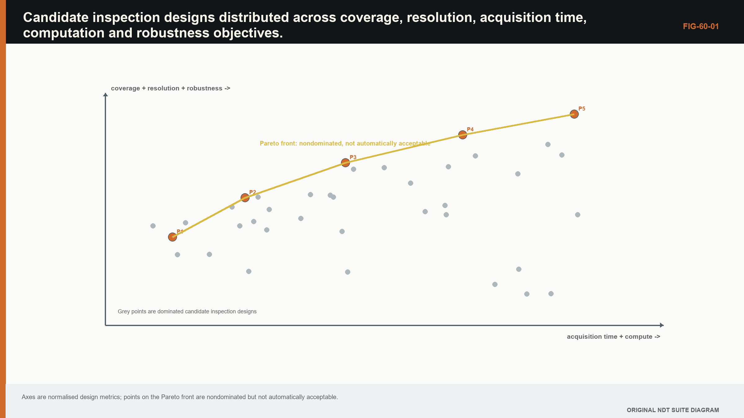
A design dominates another if it is no worse in all objectives and better in at least one, with constraints satisfied. Nondominated designs form a Pareto front. The front makes trade-offs visible without hiding them in arbitrary weights.
| (60.1) Pareto dominance for minimised objectives · EQ-60-01 Where: f_k = objective k expressed so smaller is better; A and B = feasible candidate designs Model limits: objective definitions and feasibility constraints are fixed for the comparison |
|---|
Selecting from the front requires priorities and risk. Weighting objectives can be useful, but results depend on scale and chosen weights. A sensitivity analysis over weights shows whether the choice is stable or political arithmetic wearing a lab coat.
60.10 Computational and storage constraints
Computation affects what can be used operationally. A multi-view high-resolution reconstruction may be feasible offline and impossible at scan speed. Options include reduced ROI, precomputed delays, fewer pairs, lower-resolution screening followed by refinement or distributed processing.
Storage includes raw acquisition, metadata, derived images and audit versions. Deleting raw data to meet a storage target can prevent future reprocessing and fault investigation. The information-retention requirement should be a constraint, not an afterthought.
Energy and thermal limits can matter in embedded or robotic systems. Sustained GPU performance may throttle. Benchmarks should use representative duration and data, not one warm cache run.
60.11 Validation of the selected design
Optimisation predicts a preferred design under its models. Validation tests whether the predicted advantages appear in representative data. Compare at least one alternative to avoid validating only absolute performance. Include nominal and perturbed conditions.
Commercial evaluations can inform metric design but remain bounded by the tested equipment and specimens. [R061] The final technique claim should cite its own evidence rather than the rank order of another study.
If validation contradicts optimisation, preserve the discrepancy. It may reveal wrong target scattering, noise or implementation. Retuning and retesting should use separated development and confirmation data.
| Worked example · Identifying a small Pareto set WE-60-01 Known: Three feasible designs have objective values to minimise: A = (missed-volume 2%, runtime 12 s, velocity sensitivity 1.5 mm); B = (3%, 7 s, 0.8 mm); C = (4%, 10 s, 1.2 mm). Find: Identify dominated designs. Method: B is better than C in missed volume (3% < 4%), runtime (7 < 10) and sensitivity (0.8 < 1.2), so B dominates C. A and B trade coverage against runtime and robustness, so neither dominates the other. Result: A and B form the candidate Pareto set; C can be removed under these objectives. Engineering meaning: The calculation does not choose A or B. Selection depends on the importance and uncertainty of the three metrics and any constraints not included. |
|---|
Guided Level 3 case: selecting among three technique designs
Three candidate designs cover the same weld. Design A uses a large aperture and fine grid, producing the narrowest simulated point response but the slowest processing. Design B uses more views and a moderate grid, giving stronger orientation coverage with more geometry responses. Design C uses a reduced acquisition and coarse grid, finishing quickly but showing greater coordinate change when velocity is perturbed.
Start by writing the decision need. The technique must detect planar targets across a defined orientation and position range, locate them within a stated tolerance, keep false geometry responses manageable and complete the scan within the production window. These become separate objectives and constraints. None can be replaced by a single sharpness score.
Build a small sensitivity table. For each design, perturb velocity, wedge delay, element loss, surface position and coupling within supported ranges. Measure target coordinate, response spread, signal-to-noise ratio, missed targets, false calls, processing time and data volume. Plotting each output against one input shows where the design is stable and where it has a cliff.
Reject any design that fails a mandatory constraint. The remaining designs may form a Pareto set. Design A cannot be called best merely because it has the narrowest response if it misses the scan-time constraint. Design C cannot be called best merely because it is fast if target coordinate is unstable. Design B may be preferred when its broader coverage and manageable artefacts support the actual decision, even though it wins no single metric.
Test the choice on specimens or datasets not used to tune it. Include targets near the coverage boundary and nuisance geometry that resembles them. Repeat the comparison with realistic channel loss and acquisition speed. A retrospective sparse subset must also be acquired natively before its timing and transmit conditions are accepted.
The release record preserves all candidate definitions, objective weights or decision rules, rejected alternatives and sensitivity results. It states which uncertainties were sampled and which remained outside the study. The selected technique is therefore a justified trade-off for a declared application, not a universal optimum. A later change in target population, hardware, software or production constraint triggers a defined impact review rather than silently inheriting the old choice.
60.90 Technical extension: optimisation under evidence and uncertainty
60.90.1 Constraint classification
Separate hard physical constraints, controlled operational limits and preferences. A path that cannot exist is infeasible. A storage target may be negotiable. A preferred runtime is an objective. Mixing these categories can allow an optimiser to trade away a mandatory coverage requirement for a small speed gain.
Constraints have uncertainty. If scan rate is close to its measured limit, variation can make nominally feasible designs fail. Robust feasibility evaluates the constraint across credible variation or reserves explicit margin.
60.90.2 Surrogate models
High-fidelity field and wave simulations can be too expensive for thousands of candidates. A surrogate approximates outputs from a designed set of simulations. Polynomial response surfaces, Gaussian processes and neural surrogates have different data and uncertainty behaviour.
Validate the surrogate on hold-out designs, especially near constraints and path transitions. Optimisers exploit approximation errors; the apparent best candidate should be reevaluated with the high-fidelity model and experiment.
60.90.3 Experimental design
Design-of-experiments methods select combinations that estimate main effects and interactions efficiently. Factor ranges should come from the technique model. Randomisation and replication separate drift and noise from factor response.
The response should include non-target artefacts and data-quality failures. Optimising only successful acquisitions excludes the robustness burden that production will carry.
60.90.4 Utility and consequence
When a single design must be selected, utility can represent consequence-weighted performance. The weights should be approved decision inputs, not chosen after results appear. Sensitivity to weights shows whether the decision is stable.
Expected utility can conceal rare severe outcomes. Add hard safety or coverage constraints, tail-risk measures or worst-case scenarios where consequence requires them.
60.90.5 Sequential optimisation
Optimisation can proceed in stages: screen impossible geometry, rank field support, evaluate reconstruction and artefacts, then validate finalists. This avoids spending high-fidelity effort on clearly unsuitable designs.
Stage thresholds should retain margin so early approximations do not discard a robust candidate. A traceable record shows why each candidate was removed.
60.90.6 Operational feedback
Field data can update noise, coupling and reliability models, but changes should pass governance. Production results are not automatically labelled truth. Confirmed targets, false calls and abnormal events can expand the evidence base after quality review.
An optimisation model should have version and validity range. Updating it can change the preferred technique and may trigger revalidation. [R023] [R024] [R033] [R034] [R061]
60.91 Verification of optimisation claims
Optimisation outputs should be reproducible from a candidate register containing inputs, model version, objective values and constraint status. Random or evolutionary algorithms also record seed and stopping criteria. Repeating the optimisation with another seed tests whether the apparent front is stable.
Objective uncertainty can change dominance. If two designs differ by less than model or measurement uncertainty, they should be treated as practically tied. Confidence bands or scenario envelopes around Pareto points prevent false precision.
Validate the selected design and at least one nearby alternative. If the predicted ranking reverses experimentally, investigate objective model and noise. The alternative provides information that a pass/fail test of one design cannot.
Operational constraints should be verified under sustained load, remounting, expected temperature and representative material. A design can be optimal in simulation and fragile to coupling or data throughput.
The final decision record states why one nondominated design was selected, which priorities and uncertainties were used, and what future change would invalidate the choice. This retains engineering judgement without disguising it as a mathematical inevitability. [R023] [R024] [R033] [R034] [R061]
60.92 Optimisation audit and stop rules
Define stop rules before searching: required objective convergence, maximum high-fidelity evaluations, minimum validation margin and conditions that invalidate the model. Without them, optimisation can continue until random variation produces a preferred candidate.
An audit plot shows objective history, constraint violations and diversity of candidates. A front containing nearly identical designs may indicate premature convergence. Repeating with different initial populations or algorithms tests search robustness.
After experimental validation, update model discrepancy rather than merely replacing predicted values. If the same bias appears across candidates, correct or widen the model. If ranking varies unpredictably, the optimiser lacks a reliable objective and should not drive final selection.
Operational stop rules also matter. If coupling, channel health or scan rate leaves the validated envelope, the optimised technique is no longer the same system. The acquisition should flag and preserve that boundary.
The final selected design includes fallback and contingency: acceptable reduced speed, alternate aperture after a failed element, or conditions requiring reacquisition. These options need evidence and should not be improvised under production pressure. [R023] [R024] [R061]
60.93 Optimisation evidence ledger
For the selected design, retain objectives, constraints, uncertainty scenarios, candidate front, validation results and the human decision rationale. This ledger allows a later change to show whether it moves the design off the validated trade space. Without it, the word optimal becomes an unrepeatable opinion with decimal places. [R023] [R024]
60.94 Qualification of the chosen optimum
The selected design is not qualified by being Pareto optimal. It still passes calibration, verification, representative-target and reliability evidence appropriate to its claim. Optimisation chooses what to test; qualification establishes whether it works within the declared range. [R033] [R034]
60.95 Engineering check: optimise the decision, not a single image metric
Technique optimisation is inherently multi-objective. Detection margin, resolution, coverage, scan time, data volume, artefact level and sizing stability can move in opposing directions. Collapsing them into one score is acceptable only when the weights and hard constraints are declared. Otherwise the optimiser can improve an easy metric while degrading the inspection decision that matters.
A defensible workflow first sets non-negotiable constraints, then explores the Pareto set of feasible designs. Representative target and non-target cases are evaluated with perturbations for velocity, coupling, position and channel condition. Candidate techniques are compared on confirmation data not used to tune them. The selected point should include operational margin, not merely the best nominal score. Recording rejected alternatives and the reason for selection makes later change review possible when equipment, geometry or performance requirements move. [R016] [R033] [R036] [R044]
Chapter synthesis
Technique optimisation is defined by decision outputs, constraints and uncertainty. Acquisition and reconstruction should be co-designed. Aperture, views, ROI and sampling affect target and artefact populations together. Coverage metrics need physical meaning and visible margin. Representative reflector and non-target populations prevent optimisation to one convenient target. Robust and Pareto methods expose sensitivity and trade-offs. Computation, storage and provenance are design constraints. Validation must test the predicted advantage and preserve discrepancies rather than polishing them away.
Key equations and relationships
| (60.2) Robust objective over uncertain inputs · EQ-60-02 Where: d = design; xi = uncertain inputs; J = performance loss; E = expected value; Std = standard deviation; beta = declared risk weighting Model limits: distributions of xi are defensible and mean-plus-spread represents the decision risk; interval or worst-case methods may be preferable otherwise |
|---|
In plain words
- The chapter's central control is robust design, and its meaning must be stated before its mathematics or software implementation.
- A faster, sharper or cleaner result is not automatically a more reliable result.
- Every claimed improvement depends on a declared dataset, model, configuration and target population.
- Known reference cases and deliberately difficult cases reveal different weaknesses.
- Stored raw evidence, metadata and software identity make later review possible.
- The technical conclusion must remain inside the boundary demonstrated by the evidence.
Key terms in this chapter
The words introduced at the chapter opening are the minimum vocabulary for its Level 3 work. Use them consistently in the technique, validation record and report. Where a supplier uses a different label, record the supplier term without allowing it to replace the physical definition.
Common mix-ups
- Do not confuse a similar displayed image with equivalent retained information.
- Do not confuse software verification with physical validation of an inspection technique.
- Do not confuse an assumed model output with a directly observed quantity.
- Do not confuse a demonstrated result for one target population with universal capability.
Independent review checkpoint
Give a second competent reviewer the raw or reference data, the declared robust design method, the controlled configuration and the expected comparison outputs. The reviewer should be able to reproduce the important result without using an undocumented display adjustment or private software setting. Record the version, input identity, contributor or channel mask, model inputs, numerical tolerances and any excluded cases. Also record one observation that would contradict the preferred explanation. Where the result supports a decision, the reviewer records the nearest failure boundary and one realistic change that would trigger revalidation. This checkpoint does not turn independent review into a ceremonial signature. It tests whether the evidence chain is understandable, repeatable and honest about its limits.
Bridge forward
Chapter 61 asks what evidence is required to verify, validate and establish the reliability of the selected technique.
Sources and further study
- [R016]
- [R023]
- [R024]
- [R033]
- [R034]
- [R036]
- [R044]
- [R061]
Study and revision only. This is not an approved inspection procedure, acceptance criterion or qualification.