
CHAPTER 40 · Phased Array Ultrasonics Level 3
Proving Automated Acquisition Is Complete
In this chapter · 27 sections
Why this matters
An automated scanner can finish a smooth pass while the stored PAUT data contain periodic gaps, repeated columns or one group shifted from the others. Motion, ultrasonic firing and file writing are separate activities that must remain synchronised. A lively display is not proof that complete data reached storage. A PAUT Level 3 must define what one valid spatial sample contains, calculate the rate demand, measure the system under full load and make faults visible. This chapter follows one timing strip from encoder event to committed frame, then adds clocks, queues, multiple probes, robots, recovery and release evidence.
What you already need
- Pulse repetition frequency, range, receive window and complete law sequence.
- Encoders, scan/index coordinates and maximum acquisition increment.
- Groups, probes, focal laws and stored A-scans from PAUT Level 2.
- The distinction between display refresh and acquired records.
- Basic speed, time and distance relationships.
What you will learn
- Define one complete spatial sample for an automated PAUT architecture.
- Calculate rate and latency margins using verified complete frames.
- Separate encoder resolution, accuracy, backlash and trigger timing.
- Diagnose multigroup offsets, dropped frames and queue faults from retained evidence.
- Design sustained-load, moving-reference and replay tests.
- Decide when reprocessing is valid and when missing information requires reacquisition.
Words you will meet
- Complete frame: all declared laws and groups associated with one valid spatial sample.
- Trigger: event that starts or requests an acquisition action.
- Clock domain: subsystem whose timing is controlled by one clock source.
- Latency: delay between a defined event and its resulting action.
- Jitter: variation in that delay or event timing.
- Atomic association: position and waveform paired as one indivisible record.
- Buffer: temporary memory holding data between processing stages.
- Queue: ordered set of records waiting for a downstream stage.
- Sequence counter: number used to reveal missing, duplicated or reordered records.
- Fail-detectable: designed so important faults stop, alarm or mark affected data visibly.
40.1 Build one timing strip before calculating speed
Start with one focal law. A trigger causes its pulser event, receive window and stored A-scan. A complete group contains every required law. A complete frame contains every declared group and the position assigned to that acquisition. Only after that frame is complete does one valid spatial sample exist.
This definition prevents a common rate error. An instrument may display 16,000 firings per second, while a 128-law group can form at most 125 ideal complete frames per second before receive, switching, processing and storage losses. Adding another group can halve or otherwise reduce the complete-position rate while the pulser number remains unchanged.
Choose the event that defines position. An encoder crossing may trigger the sequence. A time-based instrument sequence may run continuously while the current encoder value is sampled. A motion controller may issue a trigger only after an instrument-ready handshake. These architectures behave differently during acceleration, reversal and overload.
The following figure shows one encoder event moving through acquisition and storage.
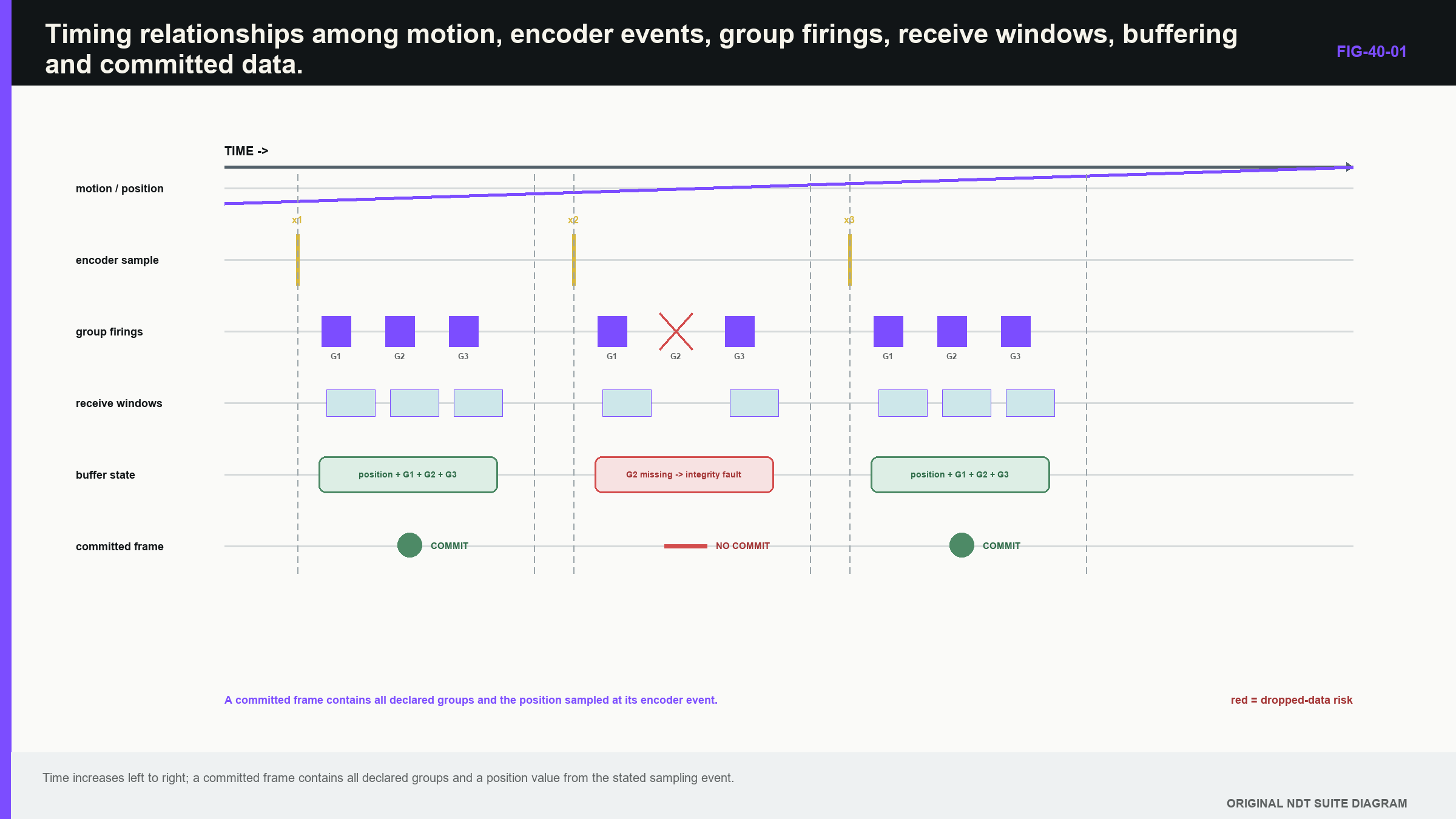
Notice that motion can remain smooth while the ultrasonic or storage branch becomes incomplete.
40.2 Choose and document the trigger architecture
In position-triggered acquisition, encoder increments request frames. This directly links spatial spacing to trigger count, but the system must manage triggers that arrive while it is busy. It may queue, inhibit, coalesce or drop them.
In time-triggered acquisition, frames run at a clocked rate and positions are attached as they occur. Spacing then grows when speed increases and shrinks when the scanner slows. At a stop, many frames can share one coordinate. Hybrid systems use motion commands, handshakes and buffered bursts.
The technique should state which event starts acquisition, when position is sampled, what happens when the system is busy and how an incomplete frame is marked. A missing frame has different meaning under each architecture. The trigger model is therefore an essential technique variable, not hidden equipment detail.
Public standards treat automated array examination as an application domain while instrument, probe and complete-system performance remain separate layers. [R042] [R043] [R044] [R045] The practical consequence is that motion, ultrasonic function and synchronisation need distinct evidence before the coupled system is accepted.
40.3 Convert scan increment into a complete-frame requirement
The physical relationship is direct: distance between complete frames equals instantaneous speed divided by verified complete-frame rate.
| (40.1) Spatial spacing from verified complete-frame rate · EQ-40-01 Where: Delta_x = along-scan spacing between complete frames (mm); v = instantaneous scan speed (mm/s); f_complete = verified fully populated frame rate (1/s) Model limits: motion is represented by the stated instantaneous speed; one valid position is paired with each complete frame; no missing or duplicated frame is hidden in the rate |
|---|
The rate requirement follows from the maximum permitted acquisition increment and the worst credible instantaneous speed, including overshoot. Design margin must cover receive windows, switching, processor load, storage delay and ordinary variation. A displayed average is insufficient if short bursts create gaps.
| Worked example · Check rate margin for an automated scan WE-40-01 Given: A setup needs 128 firings for one complete position. Allowed pulse repetition frequency (PRF) is 16,000 Hz. Intended speed is 60 mm/s, and maximum permitted complete-frame increment is 0.50 mm. Find: Compare the ideal firing-limited frame ceiling with the spatially required rate. Steps: Ideal ceiling is 16,000 firings/s / 128 firings/frame = 125 frames/s. Required rate is 60 mm/s / 0.50 mm/frame = 120 frames/s. Margin is 5 frames/s, or 5/120 x 100 = 4.2% above the requirement. Answer: The idealised ceiling is 125 frames/s against a minimum demand of 120 frames/s, leaving only about 4.2% margin. Technical implication: The design is not yet demonstrated. Receive time, switching, transfer and storage reduce usable rate, while speed overshoot raises demand. Full-load measurement or a lower released speed is required. Common mistake: Dividing speed by PRF directly or treating the fastest display update as a complete stored-frame rate. |
|---|
40.4 Range and receive time limit safe PRF
Every firing needs enough time for relevant paths to arrive and decay before another pulse can create ambiguous energy. The longest required path or slow mode can control the receive window even when most laws use shorter paths.
Multiple groups may use different ranges. Hardware recovery, receive protection and multiplexer switching add dead time. Industrial ultrasonic electronics link pulser, receiver and switching performance to repetition limits. [R015] The production rate should therefore be verified with the actual voltage, ranges, groups, averages and channel resources.
A fast PRF can create previous-pulse responses that remain believable in an automated image. A useful test varies PRF while holding geometry and position constant. A genuine reflector retains its physical time; wrap-around changes according to repetition period.
The rate budget should list firings, receive window, switching, averaging and measured system overhead. If one longest group constrains all others, redesigning group sequence or separating passes may provide more reliable margin than running at the edge.
40.5 Encoder resolution is not coordinate accuracy
Encoder resolution is distance per count. Accuracy also includes wheel diameter, calibration, slip, backlash, mounting, surface condition and path geometry. A display showing 0.01 mm counts cannot make a slipping wheel accurate to 0.01 mm.
Calibrate over representative short and long travel. Repeat in both directions to expose backlash and slip. Use the scanner, wheel pressure and surface condition that affect production. Raster scans need index-axis evidence, line identity and turn-around controls. Spiral and helical scans need angular and axial coordinates plus a component transform.
Polarity and origin must be explicit. Reversal can reveal a trigger architecture that behaves differently on negative motion. Time-triggered acquisition during acceleration changes spacing even when average line speed passes. Measure instantaneous maximum and inspect frame-to-frame increments.
Change case: new wheel material. A replacement wheel has the same nominal diameter but different compression on the component surface. Long-distance scale changes by 0.7%, while count resolution is unchanged. The affected claims include scan coordinate, response length and coverage spacing; changing the encoder scale and repeating direction/traction evidence is required.
40.6 Latency turns time into position error
An automated chain can contain motion-controller, encoder, instrument, computer and file clocks. Each is a clock domain. Equal displayed timestamps do not prove that their events are aligned.
Trigger latency is the delay between the position event and the actual acquisition. Stable latency creates a systematic offset proportional to speed. Variable latency creates jitter and spatial blur.
| (40.2) Position offset caused by fixed trigger latency · EQ-40-02 Where: Delta_x_latency = systematic coordinate offset (mm); v = scan speed (mm/s); Delta_t_latency = fixed delay from the stated position event to acquisition (s) Model limits: constant speed over the delay; stable latency; declared sign and coordinate convention |
|---|
At 100 mm/s, a 5 ms delay gives 100 mm/s x 0.005 s = 0.50 mm. Reversing direction changes the sign of a physical displacement relative to the component, which helps separate latency from encoder-scale error.
Long scans also expose clock drift. A small frequency difference accumulates between devices. Common hardware clocks or periodic alignment events can control it. Operating-system timestamps may be too uncertain for submillimetre position at high speed unless independently demonstrated.
40.7 Use a moving reference to separate scale and latency
Place a sharp known feature at an independently measured coordinate. Scan at several speeds and in both directions using the full production group count and storage destination.
A fixed latency produces displacement proportional to speed and opposite in sign on reversal. Encoder-scale error changes distance proportionally but does not produce the same direction-dependent intercept. Backlash creates a reversal-dependent local effect. This experiment turns three abstract causes into different observable patterns.
Record actual speed, sequence numbers, group completion and queue or drop counters. If the system corrects latency internally, verify the correction after firmware, controller or scanner change. Retain the raw timing evidence; a configuration tick box is not a measurement.
Evidence-boundary case. A low-speed reference pass agrees within 0.1 mm, but production speed is four times higher and no full-load test exists. The low-speed result does not support production coordinate accuracy because latency error scales with speed and queue behaviour can change under load.
40.8 Multigroup and multiple-probe systems
Groups can share pulsers, receivers and multiplexers. Enabling another group may reduce the rate available to all. State whether a reported rate is per firing, law, group or fully populated position.
Multiple probes add physical offsets and orientation transforms. One scanner coordinate can serve all groups only when each acoustic reference is transformed from the common frame. Probe reversal may change element order and skew sign. Test transforms with a common reference feature, not only mechanical drawings.
Acoustic cross-talk occurs when one probe fires before another probe's energy decays. Electrical cross-talk can enter shared electronics. Changing firing order or inter-group delay is diagnostic because interference follows timing, while a component target should remain at its corrected coordinate.
A partial frame may contain one good group and one missing group. The data format and analysis must preserve that distinction. Treating the position as complete because any group exists can create false coverage.
40.9 Immersion and robotic motion add registration chains
Immersion adds water path, temperature, stand-off and surface finding. A robot adds base frame, joint solution, tool centre, probe frame and component registration. Accurate joint repeatability does not prove acoustic coordinate accuracy.
Water velocity changes with temperature. Surface height changes incidence and refraction. Tool-centre calibration or component registration can remain wrong while the robot returns to the same point consistently. Choose independent features that test the coordinate output actually claimed.
Curved components may require probe orientation to follow the local normal. Constant nominal stand-off does not preserve incidence when tool tilt or surface shape differs from the model. Open-loop tracking uses known geometry; closed-loop tracking uses sensors. Each has different failure signatures and provenance.
The acquired surface model and its version become part of the dataset when reconstruction depends on them. A corrected image is not reproducible from waveform data alone if the geometry and registration inputs are missing.
40.10 Recognise incomplete and displaced data
Completeness checks operate at several levels:
- sequence counters reveal missing, repeated or reordered frames;
- expected law and group counts reveal partial frames;
- encoder monotonicity reveals jumps and reversals;
- channel maps reveal silent paths even when counts are complete; and
- checksums reveal corruption after acquisition.
Visual clues include periodic vertical bands, stretched or compressed regions, repeated columns, diagonal line-registration errors and group-specific shifts. These are clues rather than causes. Inspect counters, timestamps, coordinates and raw traces before diagnosis.
A deliberate pause must differ from missing data. Motion stopped while acquisition continued produces repeated positions. Acquisition stopped while motion continued produces a gap. A delayed queue flush can attach old waveforms to newer coordinates if position and data are written by separate asynchronous tasks.
Failure case: plausible interpolation. A display fills missing columns between two valid frames and shows continuous colour. Sequence counters reveal a 2.4 mm gap exceeding the 0.5 mm limit. Interpolation improves appearance but does not create inspected samples; the region remains unexamined under the released claim.
40.11 Buffers, queues and atomic position pairing
Data move from digitiser to processor, network and disk through buffers. When a downstream stage slows, a queue grows until the system throttles, drops records or fails. A short bench pass may never fill the buffer, so sustained tests must exceed the largest queue time.
Log queue occupancy, drop counters and commit latency where possible. If no counter exists, sequence numbers and expected file growth provide indirect evidence. The display often uses a decimated path and is a poor load monitor.
Position and waveform should be paired at a defined event as one atomic record. If separate processes write them, a restart or delay can attach a valid coordinate to the wrong waveform. Scan a sharp feature at different speeds and directions to expose speed-dependent pairing error.
A robust system is fail-detectable. It flags overspeed, encoder loss, buffer overflow, invalid calibration and partial frames. Silent interpolation or stale-coordinate continuation creates a more dangerous file because it remains visually plausible.
40.12 Preserve faults and decide recovery
Preserve the partial dataset, setup, logs, counters, motion history, software and firmware identities, disk state and reference checks. Deleting the failed file removes evidence about the fault boundary.
Reprocessing can correct display, filtering or a known transform when valid raw samples and metadata survive. It cannot recreate traces never acquired, restore clipped phase or prove coverage through a spatial gap. Reacquisition is required when missing information affects the claim or the fault interval cannot be bounded.
Safe abnormal-event tests should reproduce overload, communication loss, encoder slip and restart. Verify that the system stops, alarms or marks the data. Motion safety and NDT data quality are related but distinct: an emergency stop can protect people while leaving a partial dataset needing technical disposition.
40.13 Sustained-load, replay and boundary tests
Run at the maximum released combination of groups, range, sampling, voltage, speed, display load and storage destination. Continue long enough to expose queue, thermal and drift effects. Compare expected and stored positions independently at the end.
The release limit should retain margin from the first observed degradation. A passing average rate is inadequate when short bursts exceed the spatial increment. Record the maximum complete-frame spacing, not merely mean rate.
Retain a replay dataset containing encoder events, triggers, group completions, faults and file commits. Later software can be tested against overspeed, reversal, pause and partial-frame cases. Replay verifies logic but not mechanics, so pair it with periodic moving-reference and sustained-load tests.
Every stored scan should distinguish valid inspected samples, planned blank travel and invalid partial frames. Display resampling must not erase those states. The official record carries maximum verified increment and marks any exceedance.
40.14 Release test and evidence boundary
The release package states trigger architecture, position-sampling event, complete-frame content, maximum speed, verified rate, receive constraints, group sequence, encoder calibration, clock relationships, latency behaviour, probe transforms and fault controls.
It also names the operating boundary used in sustained testing. A new group, longer range, higher sampling rate, different storage computer or faster scanner can change queue and timing behaviour. Change review follows the affected mechanism rather than assuming the ultrasonic setup file controls the entire automation chain.
The final question is whether every claimed component coordinate can be traced to a fully populated acquisition and a position sampled under the released timing model. If sequence or timing evidence cannot answer that question, smooth motion and attractive images are not enough.
40.15 Integrated case: separating three overlapping faults
A raster scan shows repeated columns near each line start, a growing offset between two probes and occasional narrow blank bands. Treating all three as “encoder trouble” would hide their different mechanisms.
The repeated columns occur while the carriage accelerates under time-triggered acquisition, so several complete frames share nearly the same position. The growing probe-to-probe offset is proportional to speed and reverses sign, supporting different fixed latencies between group paths. The blank bands coincide with missing sequence numbers and high disk-queue occupancy, showing dropped complete frames under storage load.
Each fault affects a different part of the claim. Repeated positions add redundant data but can distort interpolation. Group latency affects registration and multi-view fusion. Dropped frames create genuine coverage gaps. The corrective evidence is therefore different: exclude or control acceleration regions, characterise and compensate stable group latency, and reduce load or speed until sustained acquisition retains margin.
After correction, repeat the full raster with sequence, queue and moving-reference evidence enabled. A clean final image alone cannot show that the three mechanisms were removed. The retained counters and coordinate comparison make the conclusion reproducible and define which earlier data remain invalid.
40.16 Change case: a faster storage computer
A replacement computer writes the same nominal file format and completes a short reference scan without alarms. That result supports basic compatibility, but it does not yet reproduce the released automation boundary. Driver timing, queue depth, operating-system scheduling and storage behaviour can alter burst handling even when the average write speed is higher.
Replay the controlled fault dataset to verify sequence, partial-frame and recovery logic. Then repeat the sustained moving scan at the released worst-case combination of groups, range, sample rate and speed. Compare maximum complete-frame spacing, queue occupancy, latency and file-commit sequence with the baseline.
If the new computer lowers average queue depth but introduces rare scheduling pauses, the maximum gap rather than average throughput controls the claim. The substitution is released only after the complete data path remains fail-detectable and within spatial limits. A faster specification sheet is helpful input evidence; it is not an acquisition-integrity test.
The same test should include deliberate recovery events. Pause and resume motion, reverse direction, interrupt a probe group and fill the storage path until an overload control operates. Confirm that incomplete frames carry an invalid state, sequence counters expose every gap and position association does not move to the next available waveform.
Compare both forward and reverse scans over a moving reference. A fixed trigger delay changes sign with direction, while encoder scale error does not. If the replacement computer changes scheduling jitter, the reference response broadens or becomes less repeatable even when its mean offset remains similar.
Check the final stored file rather than relying on live display counters. Some architectures acknowledge a frame before durable storage, so a clean acquisition screen can coexist with missing or reordered records after file commit. Reopen the dataset with an independent reader and reconcile declared frame count, sequence range, group population and position span.
The transfer record retains the computer, operating-system and driver identities because they form part of the demonstrated path. It also retains the measured boundary rather than promising that every future hardware upgrade will be faster. When the acquisition architecture changes, the same event-to-file reasoning determines which evidence must be repeated. [R015] [R042] [R043] [R044] [R045]
Define the production response before testing begins. At a warning threshold the scanner may slow while preserving complete frames. At a stop threshold it may halt and mark the last valid coordinate. If the system instead drops groups silently to maintain motion, the control has protected throughput by sacrificing the inspection claim.
Repeat the boundary test close to the maximum permitted speed and load rather than far below both. Record margin to the first warning, first invalid frame and sustained failure. These three points support operating limits, alarm settings and recovery instructions more effectively than one nominal pass.
Use the least favourable supported direction, acceleration state and group combination when selecting that boundary.
In plain words
- One valid spatial sample contains all required laws, groups and a position from a declared event.
- PRF and display refresh are not complete stored-frame rate.
- Encoder count resolution does not prove coordinate accuracy.
- Fixed latency creates speed-dependent position offset, while jitter creates blur.
- Multigroup and multiple-probe systems need resource budgets and coordinate transforms.
- Buffers can hide overload until a sustained run fills them.
- Missing or clipped raw information cannot be recovered by display processing.
- Automated release evidence must challenge timing, motion, storage and fault detection together.
Formal synthesis
Automated PAUT is a coupled timing, coordinate and data-integrity system. The measurement unit is a complete frame atomically associated with a declared position event. Rate and latency equations connect system timing to spatial error, while moving-reference and sustained-load tests expose behaviour not visible in static setup review. Level 3 control preserves raw fault evidence, separates recoverable processing changes from irreversible acquisition loss and releases a bounded combination of groups, ranges, motion and storage load.
Key terms
- Complete frame: full declared acquisition associated with one valid position.
- Clock domain: subsystem controlled by one timing source.
- Latency: delay from a defined trigger or position event to acquisition.
- Atomic association: inseparable pairing of waveform and position.
- Queue: records waiting for downstream processing or storage.
- Fail-detectable: design that marks or stops on significant data-quality faults.
Key relationships
- EQ-40-01 converts verified complete-frame rate and instantaneous speed into spatial spacing.
- EQ-40-02 converts fixed timing latency into systematic position offset.
- Required complete-frame rate equals worst speed divided by maximum permitted acquisition increment.
- Buffer duration and sustained load determine whether short tests can expose queue overflow.
Common mix-ups
- Pulser PRF is not complete-frame rate.
- Encoder resolution is not encoder accuracy.
- Robot repeatability is not component registration accuracy.
- A paused scanner is not the same as missing acquisition during motion.
- Interpolated pixels are not acquired spatial samples.
Bridge to Chapter 41
Chapter 40 established whether a complete dataset exists at the correct positions. Chapter 41 asks how trustworthy the numbers inside that dataset are. It treats calibration as measurement control, separates timing, sensitivity and coordinate states, and builds uncertainty only after the observable errors have been made visible.
Sources and further study
- [R015]
- [R042]
- [R043]
- [R044]
- [R045]
Study and revision only. This is not an approved inspection procedure, acceptance criterion or qualification.